The Mathematics Behind Gerrymandering – An Article by Pavan Kumar

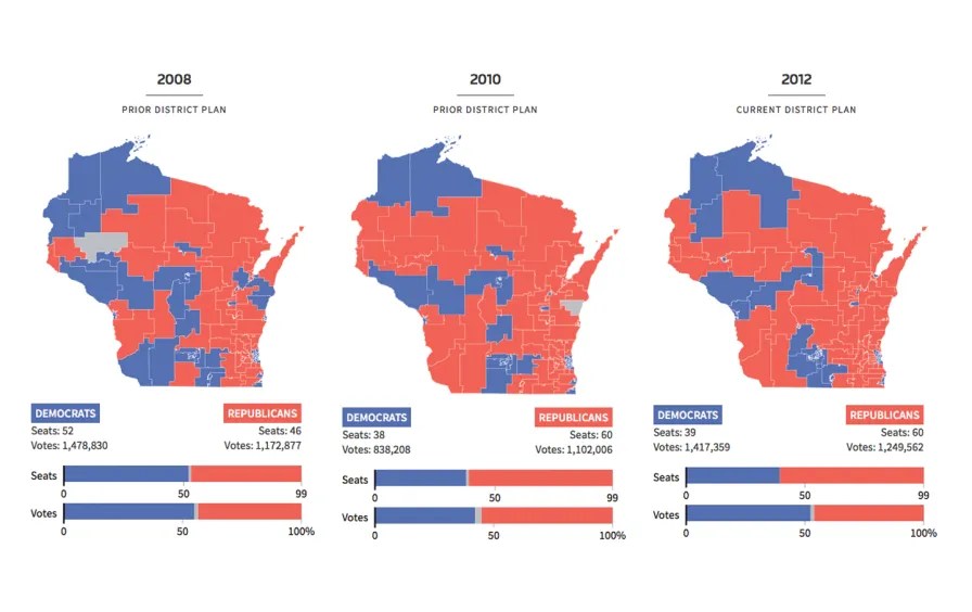
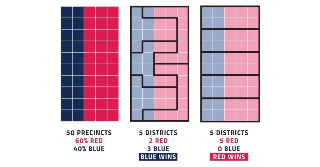
Every ten years in the United States, political figures from each state come together to redraw the boundaries of their congressional and state legislative districts. The shape of each district does not remain consistent across state lines; politicians often explain this away by stating that the districts can’t be drawn into constant shape because of how very few of the states in the U.S. are perfect squares or rectangles. The people that draw the lines vary from state to state. The way these districts are drawn are crucial because they can have huge impacts on elections, for both voters and politicians. The maps can determine the winner of elections and therefore political distribution. This can affect how communities are represented, and how accurately  they are represented. This aforementioned influence of gerrymandering proves to be a tantalizing opportunity for politicians to manipulate district lines for political gain. Although there are several political sides to gerrymandering, simple mathematics is at the heart of it for politicians. To be more specific, the mathematics behind gerrymandering comes down to two concepts: Distribution and something called the “efficiency gap”. Imagine you have a state that is composed of 4 districts and has 200 total voters. 100 of those voters align with the values of party X, and the other 100 voters align with the values of party Y. In a world with absolutely equal distribution of voters, there would be an equal amount of distribution (because of how the districts are drawn fairly) for each party, like this: 

	D1	D2	D3	D4
Party X	25	25	25	25
Party Y	25	25	25	25

Obviously, there is a complete deadlock, and as a result of that, no winner can be declared. This is why districts are not drawn completely “fairly”, they are almost always drawn with a bias for one political party over the other. If there was a bias for party X when drawing district lines, the distribution would look like this:

	D1	D2	D3	D4
Party X	20	20	20	40
Party Y	10	10	10	70

Although there is a concession in D4 to party Y, party X still wins ¾ of the races in the districts, so that means Party X wins the overall election, giving party X the political power they desired when manipulating district lines. If there was a bias for party Y when drawing district lines, the distribution could look like this:

	D1	D2	D3	D4
Party X	10	10	10	70
Party Y	35	35	27	3

The same occurs here, with there being one concession to party X, however, party Y wins ¾ of the races and thus wins the overall election. 

The second concept that is tied closely to gerrymandering is the concept of the efficiency gap. The efficiency gap is essentially the difference between the two parties’ “wasted” votes divided by the total number of votes. Votes have different amounts of power depending on the state. Right now, in California, a vote for or against the Democratic party does not hold as much as a vote in a battleground state such as Florida. This is because of how the Democratic party has consistently won California for several years now, so Republican voters in California have much less power with their vote, on top of this, votes for the Democratic party in California don’t hold as much power either because of the sheer dominance of the Democratic party in California. If the Democratic party wins California by 65% or 55%, the result remains the same (a Democratic win), so the extra winning votes are essentially wasted. In other words, wasted votes can go to the winning candidate, as well as the losing candidate. To demonstrate the determination of the efficiency gap, we can look at the previous distribution (of voters) table that favored party Y. Here, 65 of party x’s votes are wasted, 30 of them in losing causes and 35 of them coming from winning D4’s election by 35 more votes than the 25 benchmark. For party Y, 25 votes are wasted. By doing (65-25) then dividing it by the total number of votes in the election (200), we can find the efficiency gap. In this scenario, 20% of the wasted votes favor party Y, and the same is true for party X in the first distribution scenario. 

From here, we can begin to think about how we can make elections more “fair” (without the bias that comes with politicians drawing the district lines every ten years), using the efficiency gap. It is widely thought that when the efficiency gap is lower in percentage, the election can be determined to be more “fair”. Thus, the most fair election possible is a scenario where the efficiency gap is at 0%, for example (with a state with 10 districts and 400 total voters): 

	D1	D2	D3	D4	D5	D6	D7	D8	D9	D10
Party X	30	30	30	30	30	10	10	10	10	10
Party Y	10	10	10	10	10	30	30	30	30	30

In this situation, both sides waste the same amount of votes, so therefore, the efficiency gap will be at 0%. In this scenario, neither party wins the overall election, they each win an equal amount of district elections, which is the ideal outcome of a mathematically “fair” election. Armed with this, politicians and mathematicians of the future can begin to use the efficiency gap as a concept to measure electoral fairness, and make changes so that more of America’s communities are represented fairly.